Bayesian Inference Priors, Posteriors, Conjugates Cheat Sheet

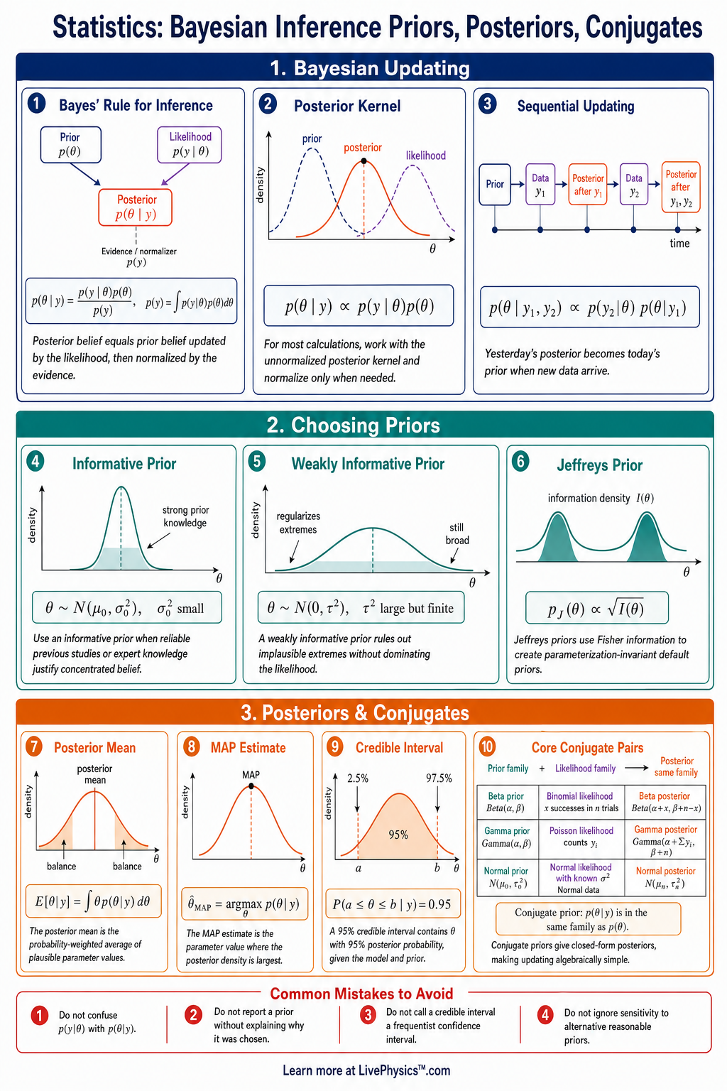
A printable reference covering Bayes' theorem, priors, likelihoods, posteriors, conjugate families, posterior means, and credible intervals for college.

Download PNG

Related Tools

Related Labs

Related Worksheets

Related Infographics

Bayesian inference updates beliefs about unknown parameters using observed data. This cheat sheet covers priors, likelihoods, posteriors, posterior summaries, and common conjugate prior models. Students need it because Bayesian calculations often become simpler when the right prior family is matched to the likelihood. It is designed as a quick reference for interpreting formulas and choosing standard models. The central rule is Bayes' theorem, which says the posterior is proportional to the likelihood times the prior. A prior distribution encodes information before seeing the data, while the likelihood measures how compatible parameter values are with the observed data. Conjugate priors make the posterior stay in the same distribution family as the prior, which gives closed-form updates. Posterior means, variances, predictive distributions, and credible intervals summarize the updated uncertainty.

Key Facts

Bayes' theorem for a parameter is $p(\theta \mid y)=\frac{p(y \mid \theta)p(\theta)}{p(y)}$ , where $p(y)=\int p(y \mid \theta)p(\theta)\,d\theta$ .
The posterior kernel is $p(\theta \mid y) \propto p(y \mid \theta)p(\theta)$ , so constants not involving $\theta$ can be ignored during proportional calculations.
For $Y \mid \theta \sim \operatorname{Binomial}(n,\theta)$ and $\theta \sim \operatorname{Beta}(\alpha,\beta)$ , the posterior is $\theta \mid y \sim \operatorname{Beta}(\alpha+y,\beta+n-y)$ .
For $Y_i \mid \lambda \sim \operatorname{Poisson}(\lambda)$ and $\lambda \sim \operatorname{Gamma}(\alpha,\beta)$ using rate $\beta$ , the posterior is $\lambda \mid y \sim \operatorname{Gamma}(\alpha+\sum_i y_i,\beta+n)$ .
For $Y_i \mid \mu \sim N(\mu,\sigma^2)$ with known $\sigma^2$ and $\mu \sim N(\mu_0,\tau_0^2)$ , the posterior variance is $\tau_n^2=\left(\frac{1}{\tau_0^2}+\frac{n}{\sigma^2}\right)^{-1}$ .
For the normal mean model with known $\sigma^2$ , the posterior mean is $\mu_n=\tau_n^2\left(\frac{\mu_0}{\tau_0^2}+\frac{n\bar{y}}{\sigma^2}\right)$ .
A $95\%$ credible interval for $\theta$ is an interval $[a,b]$ such that $P(a \le \theta \le b \mid y)=0.95$ .
The posterior predictive distribution is $p(\tilde{y} \mid y)=\int p(\tilde{y} \mid \theta)p(\theta \mid y)\,d\theta$ .

Vocabulary

Prior distribution: A probability distribution $p(\theta)$ that represents uncertainty about a parameter before observing the current data.
Likelihood: The function $p(y \mid \theta)$ that measures how plausible the observed data are for each possible value of $\theta$ .
Posterior distribution: The updated distribution $p(\theta \mid y)$ for a parameter after combining the prior distribution with the likelihood.
Conjugate prior: A prior distribution that produces a posterior distribution in the same family after being updated by a specified likelihood.
Marginal likelihood: The normalizing constant $p(y)=\int p(y \mid \theta)p(\theta)\,d\theta$ that makes the posterior integrate to $1$ .
Credible interval: An interval that contains the parameter with a stated posterior probability, such as $P(a \le \theta \le b \mid y)=0.95$ .

Common Mistakes to Avoid

Confusing the likelihood with the posterior is wrong because $p(y \mid \theta)$ is a function of $\theta$ based on fixed data, while $p(\theta \mid y)$ is a probability distribution over $\theta$ .
Dropping terms that contain the parameter is wrong because only constants independent of $\theta$ can be ignored when using $p(\theta \mid y) \propto p(y \mid \theta)p(\theta)$ .
Mixing Gamma rate and scale conventions is wrong because $\operatorname{Gamma}(\alpha,\beta)$ with rate $\beta$ has mean $\frac{\alpha}{\beta}$ , while using scale gives mean $\alpha\beta$ .
Interpreting a frequentist confidence interval as a Bayesian credible interval is wrong because a credible interval makes a probability statement about $\theta$ conditional on the observed data.
Using a conjugate update without checking the likelihood form is wrong because conjugacy depends on the exact sampling model, such as Binomial with Beta or Poisson with Gamma.

Practice Questions

1 Let $Y \mid \theta \sim \operatorname{Binomial}(20,\theta)$ and $\theta \sim \operatorname{Beta}(3,5)$ . If $y=14$ , find the posterior distribution of $\theta$ .
2 Let $Y_1,\ldots,Y_5 \mid \lambda \sim \operatorname{Poisson}(\lambda)$ with observations $2,0,3,1,4$ , and let $\lambda \sim \operatorname{Gamma}(2,3)$ using rate $3$ . Find the posterior distribution of $\lambda$ .
3 For $Y_i \mid \mu \sim N(\mu,4)$ with known variance $4$ , prior $\mu \sim N(10,9)$ , sample size $n=16$ , and sample mean $\bar{y}=12$ , compute $\tau_n^2$ and write the formula for $\mu_n$ .
4 Explain why a very concentrated prior can strongly influence the posterior even when the likelihood is based on real data.

Sign in to save