Click image to open full size
Differential Equations and Slope Fields Cheat Sheet
A printable reference covering differential equations, slope fields, separation of variables, exponential growth, and logistic models for grades 11-12.
Related Tools
Related Labs
Related Worksheets
Related Infographics
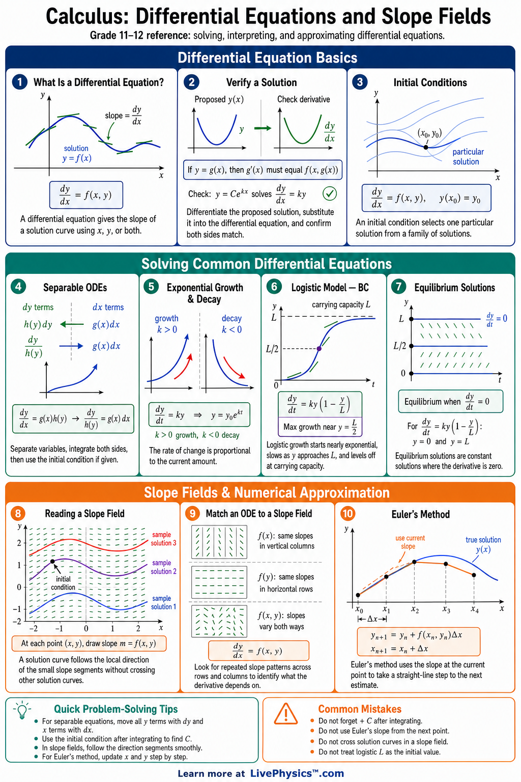
Differential equations describe relationships between a function and its rate of change. In calculus, they are used to model motion, population growth, cooling, mixing, and many other changing quantities. This cheat sheet helps students connect symbolic equations, graphical slope fields, and solution curves. It is especially useful for AP Calculus and precalculus students beginning differential equation models. The most important idea is that a differential equation such as gives the slope of a solution curve at each point. A slope field shows many small tangent segments that guide the shape of possible solutions. Some differential equations can be solved by separating variables and integrating both sides. Common models include exponential growth or decay, , and logistic growth, .
Key Facts
- A first-order differential equation has the form and gives the slope of at each point .
- A slope field is made by drawing a short line segment with slope at many points in the coordinate plane.
- A solution curve to must be tangent to the slope field segment at every point it passes through.
- A separable differential equation can be written as , then solved by integrating .
- The general solution of exponential growth or decay is , where is the initial amount when .
- If in , the model shows growth, and if , the model shows decay.
- The logistic differential equation has carrying capacity and grows fastest when .
- An initial condition such as selects one particular solution from a family of solutions.
Vocabulary
- Differential Equation
- An equation involving a function and one or more of its derivatives, such as .
- Slope Field
- A graph of short line segments showing the slope given by at many points.
- Solution Curve
- A curve whose tangent slope at every point matches the differential equation.
- Separation of Variables
- A method for solving some differential equations by placing all terms with and all terms with .
- Initial Condition
- A given value such as that determines a specific solution from the general solution.
- Equilibrium Solution
- A constant solution where the derivative is zero, such as .
Common Mistakes to Avoid
- Treating a slope field segment as a point value is wrong because the segment shows the local slope, not the height of the solution.
- Forgetting the constant of integration is wrong because solving gives a family of solutions until an initial condition is applied.
- Separating variables incorrectly is wrong because every factor containing must stay with and every factor containing must stay with .
- Drawing solution curves that cross is wrong for most basic first-order differential equations because one point cannot have two different solution directions.
- Assuming exponential growth for every population model is wrong because logistic models include a limiting carrying capacity .
Practice Questions
- 1 For , find the slope of the solution curve at the point .
- 2 Solve the separable differential equation with initial condition .
- 3 A population satisfies . Find the carrying capacity and the population size where growth is fastest.
- 4 Explain how a slope field can show whether solutions are increasing, decreasing, or approaching an equilibrium solution without solving the differential equation.