3D Vector Field Explorer
Build intuition for 3D vector calculus. Plot any field F(x, y, z), move a probe through it, and read off the divergence and curl numerically. Includes presets for rotational, radial, and dipole patterns.
Probe at (1.000, 1.000, 0.000)
Drag to orbit. Scroll to zoom. X axis is red, Y is green, Z is blue. Arrows show the vector field F(x, y, z) at grid points. Edit the component expressions to explore your own fields.
Controls
Field components F(x, y, z)
Display
Probe
Presets
Reference Guide
Vector Field
A vector field assigns a vector to every point of space.
Examples include velocity in a fluid, gravitational acceleration, and the electric field. Use mathjs syntax for expressions (sqrt, sin, exp, ^ for powers).
Divergence
The divergence measures how much the field locally spreads outward (or sinks in).
Positive divergence indicates a source, negative a sink. Pure rotational fields have zero divergence everywhere.
Curl
The curl measures the local rotation of the field.
Conservative fields (gradients) have zero curl. The classic F = (-y, x, 0) has constant curl (0, 0, 2).
Helmholtz Decomposition
Any smooth vector field can be written as the sum of a gradient and a curl
This separates the irrotational part from the solenoidal part. It underlies the existence of both V (potential) and A (vector potential) in electromagnetism.