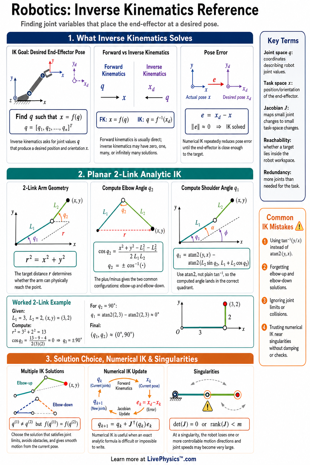
Inverse kinematics is the process of finding the joint variables that move a robot end-effector to a desired position and orientation. Students need this reference because IK problems connect geometry, algebra, trigonometry, matrices, and physical robot limits. A cheat sheet helps organize the main formulas, solution methods, and warnings used in robotics classes and projects.
Key Facts
- Forward kinematics maps joint variables to pose using x = f(q), where q is the vector of joint variables and x is the end-effector pose.
- Inverse kinematics solves q = f^-1(x_desired), but a robot may have zero, one, or many valid joint solutions for the same pose.
- For a planar 2-link arm, r^2 = x^2 + y^2 and cos(theta2) = (r^2 - L1^2 - L2^2) / (2 L1 L2).
- For a planar 2-link arm, theta1 = atan2(y, x) - atan2(L2 sin(theta2), L1 + L2 cos(theta2)).
- A target is unreachable if its distance from the base is greater than L1 + L2 or less than abs(L1 - L2) for a 2-link planar arm.
- The Jacobian relates joint velocity to end-effector velocity using x_dot = J(q) q_dot.
- A singularity occurs when det(J) = 0 for a square Jacobian, meaning the robot loses at least one direction of controllable motion.
- Numerical IK often updates joints with q_new = q_old + alpha J_pinv e, where e is pose error, J_pinv is the pseudoinverse, and alpha is a step size.
Vocabulary
- Inverse kinematics
- The method of calculating joint variables needed to place a robot end-effector at a desired pose.
- Forward kinematics
- The method of calculating the end-effector pose from known joint variables and robot geometry.
- End-effector
- The tool, gripper, sensor, or final link of a robot that interacts with the environment.
- Pose
- The combination of position and orientation that describes where an object is and how it is rotated.
- Jacobian
- A matrix that relates small changes or velocities in joint variables to changes or velocities of the end-effector.
- Singularity
- A robot configuration where motion control becomes limited because the Jacobian loses rank.
Common Mistakes to Avoid
- Using degrees when a calculator or program expects radians, which gives incorrect sine, cosine, and atan2 values.
- Assuming every target has one IK solution, which is wrong because many robot arms can reach the same pose with elbow-up, elbow-down, or other configurations.
- Ignoring reach limits, which is wrong because the equations may produce invalid values such as cos(theta2) greater than 1 or less than -1.
- Forgetting joint limits, which is wrong because a mathematical solution may require a joint angle the real robot cannot physically reach.
- Treating a singularity as just a small error, which is wrong because the robot may lose control in a direction or require very large joint speeds.
Practice Questions
- 1 A planar robot arm has L1 = 4 cm and L2 = 3 cm. Can it reach a target at x = 6 cm, y = 0 cm? Explain using the reach limits.
- 2 For a 2-link planar arm with L1 = 5 cm, L2 = 5 cm, x = 6 cm, and y = 8 cm, compute r and decide whether the target is reachable.
- 3 For a 2-link planar arm with L1 = 3 m, L2 = 2 m, x = 4 m, and y = 1 m, calculate cos(theta2) using cos(theta2) = (x^2 + y^2 - L1^2 - L2^2) / (2 L1 L2).
- 4 Why can inverse kinematics have multiple valid answers for the same end-effector pose, and why must a robot controller choose carefully among them?
Understanding Inverse Kinematics Reference
Robot geometry is built from coordinate frames. A frame gives an origin and directions for measuring position. Each link carries its own frame, and each joint changes the frame of every link beyond it.
Rotating a joint near the base affects the whole arm. Rotating a wrist joint mainly changes the tool direction. This is why a robot program must keep track of both location and orientation.
A gripper may reach the right point but still fail if it approaches at the wrong angle. In three dimensions, orientation is harder than position because rotations can be described in several ways, each with its own limits.
A desired tool pose does not usually point to one obvious arm shape. A simple elbow can bend in two different directions while placing the hand in the same spot. More complex arms may have many choices because extra joints give extra freedom.
The controller must choose a solution using practical rules. It may prefer the solution closest to the current posture, one that avoids a table, or one that stays away from joint limits.
A mathematically valid pose is not automatically safe. Real robots have cable routes, mechanical stops, payload limits, and nearby objects that the geometric model may not include.
The Jacobian is especially useful when a robot is already moving. It describes how small joint motions produce a small tool motion at the current arm configuration. This local description is used for smooth tracking, joystick control, and force control.
Near a singularity, different joint motions can produce nearly the same tool motion. The arm then needs very large joint speeds to move the tool in certain directions. Motors can saturate, motion can become jerky, and small sensor errors can cause large changes in the calculated joint command.
A good motion planner avoids these postures when possible. It may slow the robot down or choose a different arm shape.
Many real systems use numerical inverse kinematics instead of solving every geometry problem by hand. The program begins with a trial joint configuration. It measures the difference between the current pose and the target pose, then makes a small correction.
This repeats until the error is small enough or a stopping limit is reached. The correction size matters. Large steps can overshoot or oscillate.
Very small steps can make motion slow. The starting configuration matters too, since the same target can lead to different final postures. Numerical methods can fail for unreachable targets, tight joint limits, or targets near singularities, so software needs checks rather than assuming every request will succeed.
Students often lose marks through small setup errors. Keep track of whether angles use degrees or radians. Use one consistent positive rotation direction.
Draw the base frame and every link before writing equations. Test a model with easy cases, such as an arm fully stretched or folded. Then compare the calculated joint values by putting them back into the forward model.
In a classroom robot, watch the actual motion at low speed first. A result that looks correct on paper can still reveal a reversed motor direction, an offset encoder, or a frame placed in the wrong location.