Chaos & Logistic Map Lab
One simple rule, x next = r·x·(1 − x), turns a single growth rate into a journey from a steady value, through doubling cycles, into chaos. Move the growth rate r and watch the orbit, the cobweb, and the bifurcation diagram redraw.
Guided Experiment Follow the period-doubling cascade from r = 3 into chaos, then find the period-3 window.
The logistic map has a single stable value for r between 1 and 3. Predict what happens to the number of values in the long run orbit as you raise r past 3, and predict the sign of the Lyapunov exponent once the orbit becomes chaotic.
Write your hypothesis in the Lab Report panel, then click Next.
Controls
The gap between the two starting values in the sensitivity plot. A tiny gap of 0.000001 is enough to grow into a large difference once the map is chaotic.
Cobweb diagram
The parabola y = r·x·(1 − x) (teal), the line y = x (gray), and the staircase iteration path (red) from x0.
Bifurcation diagram (the Feigenbaum picture)
For each growth rate r the long run attractor values are plotted. The single line splits into 2, 4, 8, then a chaotic smear, with periodic windows inside. The red line marks your current r.
Orbit (x against step n)
The value of x at each iteration. A flat line is a fixed point, a zigzag is a cycle, and a scatter is chaos.
Sensitivity to initial conditions
Two orbits that start a gap of 0.000001 apart. In chaos they separate to order 1 (the butterfly effect, linked to a positive Lyapunov exponent). When stable they fall back together.
Data Table
(0 rows)| # | Growth rate r | x0 | Behavior | Lyapunov λ | Distinct values | Fixed point x* |
|---|
Reference Guide
The Logistic Map
The logistic map is a population model in discrete time. Each year the fraction x of the maximum population updates by a single rule.
x next = r·x·(1 − x)
Here x stays between 0 and 1 and the growth rate r runs from 0 to 4. The term (1 − x) limits growth when the population gets crowded.
The Fixed Point and Its Stability
A fixed point is a value that maps to itself. For r above 1 the nonzero fixed point is x* = 1 − 1/r.
- For r between 1 and 3 the fixed point is stable and the orbit settles onto it.
- The map's slope at x* is 2 − r. The fixed point stays stable while that slope has size below 1.
- At r = 3 the slope reaches size 1 and the fixed point loses stability.
The Period-Doubling Cascade
Past r = 3 the single value splits into a repeating cycle, and each split happens at a smaller and smaller gap in r.
- r = 3. Period 2 begins. The orbit alternates between two values.
- r ≈ 3.449. Period 4 begins.
- r ≈ 3.544. Period 8 begins, then period 16, and so on.
The shrinking gaps approach a limit by the Feigenbaum constant of about 4.669, the ratio of one gap to the next.
The Onset of Chaos
The doublings pile up at the accumulation point near r ≈ 3.5699. Beyond it the orbit no longer settles into any short cycle.
- For r above about 3.5699 the map is chaotic over most of the range.
- The orbit visits a whole band of values and never exactly repeats.
- The same rule, with no random input, produces unpredictable looking output.
The Bifurcation Diagram
The bifurcation diagram plots the long run attractor for every growth rate r at once. It is the headline picture of the route to chaos.
- A single curve for stable r, then a fork at each period doubling.
- A dense smear where the map is chaotic.
- Clear gaps inside the chaos are periodic windows.
The whole figure is self similar. Zooming into a fork reveals the same branching pattern again.
Periodic Windows
Chaos is not the whole story above r ≈ 3.5699. Narrow bands of r restore clean cycles inside the chaotic region.
- The most famous is the period-3 window near r ≈ 3.83.
- Each window begins suddenly and then doubles its own way back into chaos.
- A theorem of Sharkovskii links period 3 to the presence of every other period.
The Lyapunov Exponent
The Lyapunov exponent λ measures how fast two nearby orbits move apart, on average, per step.
λ = average of ln|r·(1 − 2·x)| along the orbit
A negative λ means nearby orbits pull together, the sign of a stable cycle. A positive λ means they separate exponentially, the signature of chaos.
Sensitive Dependence
In the chaotic regime a tiny difference in the starting value grows into a large difference, often called the butterfly effect.
- Two orbits starting 0.000001 apart can fully separate within tens of steps.
- The separation rate matches a positive Lyapunov exponent.
- Long range prediction becomes impossible even though the rule is exact.
When the map is stable instead, the same pair of orbits reconverges to the fixed point and the gap vanishes.