Biot-Savart Magnetic Field Line Visualizer
Explore how moving charges and currents generate magnetic fields. Adjust source geometry, currents, and probe positions to see field lines, vector arrows, and magnitude heatmaps update from the Biot-Savart law.
Click anywhere to move the probe (orange marker). Vector arrows always indicate the local B field direction.
Probe Reading
Controls
Display
Presets
Reference Guide
Biot-Savart Law
Every current element contributes a small field perpendicular to itself and to the displacement vector to the probe point.
The total field is obtained by integrating over the entire current path. The vacuum permeability is .
Long Straight Wire
For an infinitely long, straight wire carrying current I, the field encircles the wire (right-hand rule).
Doubling the distance halves the field. The direction is azimuthal, perpendicular to both the wire and the radial vector.
Circular Loop on Axis
Along the axis of a circular loop of radius R carrying current I, the field falls off like a dipole.
At the center (z = 0) the field reduces to . Far away it decays as .
Ideal Solenoid
For a long, tightly wound solenoid with n turns per unit length, the interior field is uniform.
Outside an ideal solenoid the field is essentially zero. Real solenoids have weak fringing fields near the ends.
Helmholtz Coil Pair
Two coaxial coils of radius R separated by distance R produce a remarkably uniform field at the midpoint.
Used for sensitive experiments needing low-gradient calibrated fields, like cancelling Earth's field.
Parallel Wire Force
Two parallel wires carrying currents and separated by d exert a force per unit length on each other.
Same-direction currents attract. Opposite currents repel. This relationship historically defined the ampere.