Click image to open full size
Linear Regression Inference Cheat Sheet
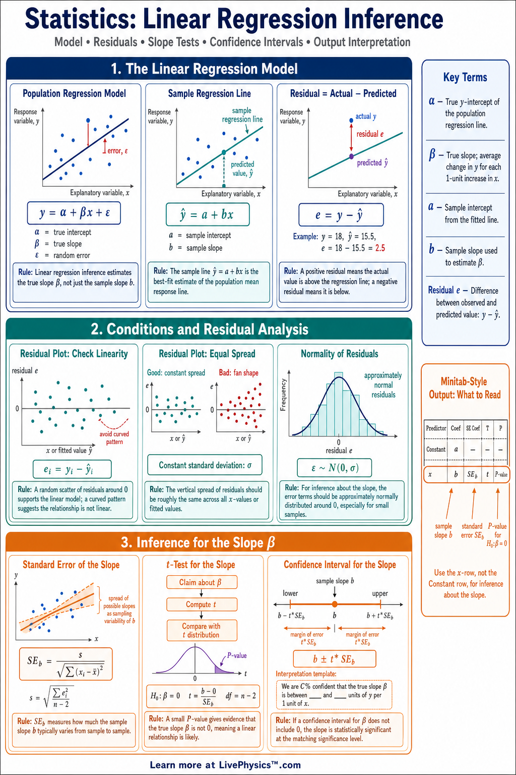
A printable reference covering regression slope tests, confidence intervals, residual standard error, conditions, and prediction intervals for grades 11-12.
Related Tools
Related Labs
Related Worksheets
Related Infographics
Linear regression inference helps students decide whether a linear relationship in sample data gives evidence of a real relationship in the population. This cheat sheet covers inference for the slope, including confidence intervals, hypothesis tests, conditions, and interpretation. It is useful when students already know how to fit a least-squares regression line and now need to make conclusions beyond the sample data. The main parameter is the population slope , which describes the average change in the response variable for each -unit increase in the explanatory variable. Inference uses the sample slope , its standard error , and a distribution with . Students must check linearity, independence, normality of residuals, and equal variability before trusting a confidence interval or significance test.
Key Facts
- The population regression model is , where is the intercept and is the slope.
- The least-squares regression line is , where and estimate and .
- The residual standard error is , which estimates the typical vertical prediction error.
- The standard error of the slope is .
- A confidence interval for the population slope is with .
- The test statistic for testing is with .
- The four main conditions are linear pattern, independent observations, approximately normal residuals, and roughly constant residual spread.
- A small -value gives evidence against , meaning the data suggest a linear relationship in the population.
Vocabulary
- Population slope
- The population slope is the true average change in the mean response for each -unit increase in the explanatory variable.
- Sample slope
- The sample slope is the slope of the least-squares regression line computed from sample data.
- Residual
- A residual is the difference between an observed value and its predicted value, written as .
- Standard error of the slope
- The standard error measures the typical sampling variability of the sample slope .
- Degrees of freedom
- For linear regression inference, the degrees of freedom are because two parameters, and , are estimated.
- Prediction interval
- A prediction interval estimates a likely range for an individual future response value at a given explanatory value.
Common Mistakes to Avoid
- Interpreting as proof of causation is wrong because regression inference can show association, but causation requires a well-designed experiment or strong causal evidence.
- Using regression inference without checking residual plots is wrong because curved patterns, outliers, or changing spread can make the procedures unreliable.
- Forgetting that is wrong because linear regression estimates both an intercept and a slope before calculating residual variation.
- Interpreting a confidence interval for as a range for is wrong because it estimates the population slope, not individual response values.
- Extrapolating far beyond the observed -values is wrong because the linear pattern may not continue outside the range of the data.
Practice Questions
- 1 A regression analysis gives , , and . Compute the test statistic for and state the degrees of freedom.
- 2 A sample gives , , and . If , find a confidence interval for .
- 3 For a regression with , the residual sum of squares is . Compute the residual standard error .
- 4 A residual plot shows a clear curved pattern. Explain why a linear regression inference procedure for may not be appropriate.