Linear Programming Lab
Work through real-world optimization problems using the graphical method. Set up objective functions and constraints, visualize feasible regions, identify optimal solutions, and explore how changing parameters affects the answer.
Guided Experiment Graphical Method
Where do you predict the optimal solution will be found, at a corner point, on an edge, or in the interior of the feasible region?
Write your hypothesis in the Lab Report panel, then click Next.
Feasible Region
Controls
Results
Corner Points
| x | y | Z |
|---|---|---|
| 3.00 | 1.50 | ★ 21.00 |
| 4.00 | 0.00 | 20.00 |
| 0.00 | 3.00 | 12.00 |
| 0.00 | 0.00 | 0.00 |
Data Table
(0 rows)| # | Problem | Constraints | Corner Pts | Optimal x | Optimal y | Optimal Z |
|---|
Reference Guide
LP Formulation
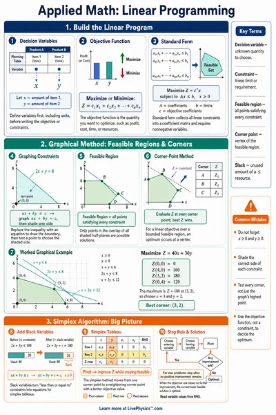
Every linear program has three parts, decision variables, an objective function, and constraints.
The objective coefficients represent profit, cost, or some other quantity to be maximized or minimized.
Graphical Method
For two-variable problems, the graphical method plots each constraint as a line and identifies the feasible region.
The optimal solution is found by evaluating the objective at each corner point of the feasible polygon.
Corner Point Theorem
If a linear program has an optimal solution, it occurs at a vertex (corner point) of the feasible region.
This theorem makes it possible to solve LP problems by checking a finite number of points.
Binding Constraints
A constraint is binding when it holds with equality at the optimal solution. Non-binding constraints have slack.
Only binding constraints affect the optimal value. Relaxing a non-binding constraint does not change the solution.