Neural Network Playground
Choose the number of hidden layers and neurons, an activation function, a learning rate, and a 2D dataset. Press Run Experiment and watch the network train one epoch at a time. The shaded heatmap shows the predicted class everywhere on the plane, so you can see a hidden layer bend the boundary around shapes that a single straight line cannot separate.
Guided ExperimentCan a single layer separate the circle dataset?
The circle dataset puts one class in an inner disk and the other in an outer ring. Predict whether a network with no hidden layer, which behaves like logistic regression, can separate them. What accuracy do you expect?
Write your hypothesis in the Lab Report panel, then click Next.
Decision Boundary
Training Metrics
- Press Run Experiment to train the network and watch the boundary form.
- The shaded heatmap shows the predicted class at every point on the plane.
Network Structure
Controls
Range 1 to 3
Data Table
(0 rows)| # | Dataset | Hidden layers | Neurons | Activation | Learn rate | Accuracy |
|---|
Reference Guide
What a Neural Network Is
A neural network is a stack of layers. Each layer takes the numbers from the layer before it, multiplies them by weights, adds a bias, and passes the result through an activation function.
- The input layer holds the two features of each point.
- Hidden layers learn useful combinations of the inputs.
- The output layer gives a probability between 0 and 1.
Why Hidden Layers Bend the Boundary
A model with no hidden layer can only draw one straight cut, just like logistic regression. It fails on the circle, moons, and spiral datasets.
A hidden layer combines several simple lines through a nonlinear activation. Stacking those pieces lets the network draw curved and even closed boundaries, so it can wrap a region around the inner disk of the circle dataset.
More neurons and more layers give the boundary more flexibility, which helps on harder shapes such as the spiral.
Training, Loss, and Backpropagation
Training minimizes the mean binary cross-entropy loss, which is small when correct points get high probability.
Backpropagation computes how each weight affects the loss, and gradient descent nudges every weight a small step in the direction that lowers it. One epoch is one full pass over the dataset.
Learning Rate and Activation Choices
- A small learning rate trains smoothly but slowly. A large rate trains fast but can make the loss bounce or fail to settle.
- tanh and ReLU usually train faster than sigmoid, whose gradients shrink far from zero.
- ReLU often produces sharp, angular boundaries, while tanh and sigmoid produce smoother curves.
- Adding noise spreads the points out and makes a clean boundary harder to find.