PCA Dimensionality Reduction Lab
Principal component analysis finds the directions a dataset varies along the most. Build a 2D cloud, then watch PCA recover its principal axes as the eigenvectors of the covariance matrix, and measure how much variance you keep when you compress the cloud from two dimensions down to one.
Guided ExperimentWhen does projecting 2D data onto one axis lose almost no information?
Predict how the explained variance of PC1 changes as you make the cloud thinner. Start from a round blob where sigma1 and sigma2 are close, then increase sigma1 while shrinking sigma2. Predict at what shape PC1 starts to keep more than 90 percent of the variance.
Write your hypothesis in the Lab Report panel, then click Next.
Controls
Each new sample draws a fresh random cloud with the same shape, so the points move a little while the principal components stay close. The projection axis lets you measure how much variance any direction captures, which peaks exactly along PC1.
Point cloud and principal axes
Variance captured vs projection angle
The projected variance is maximized exactly at the PC1 angle (30°) and minimized 90° away. The amber dot marks your projection axis at 30°.
Principal components
PC1 explained variance
89.8%
share captured by PC1
PC2 explained variance
10.2%
share captured by PC2
Eigenvalue lambda1
9.03
variance along PC1
Eigenvalue lambda2
1.03
variance along PC2
PC1 direction
29.9°
angle of the major axis
Reconstruction error (1D)
10.2%
variance lost dropping PC2
Your projection axis
At 30° the projected variance is 9.03, which is 100% of the PC1 maximum (9.03) and 90% of the total variance.
Variance along any axis is largest exactly at the PC1 angle of 29.9° and smallest 90° away at the PC2 angle.
The math
Explained variance ratio PC1 = lambda1 / (lambda1 + lambda2) = 9.03 / 10.06 = 89.8%
Reconstruction error (1D) = lambda2 / (lambda1 + lambda2) = 10.2%
Data Table
(0 rows)| # | sigma1 | sigma2 | theta (deg) | points | lambda1 | lambda2 | PC1 explained % | PC1 angle (deg) |
|---|
Reference Guide
What PCA Does
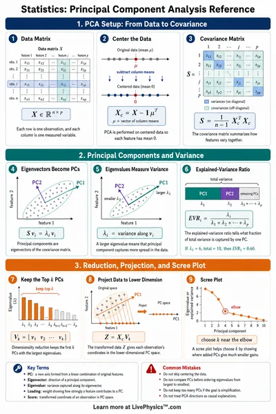
Principal component analysis rotates the coordinate axes to line up with the directions of greatest variance in the data. The first principal component points along the longest spread, and each later component is perpendicular to the ones before it.
- PC1. The direction of maximum variance.
- PC2. Perpendicular to PC1, holding the leftover variance.
- Goal. Re-express the data in fewer axes that still carry most of the spread.
The Covariance Matrix
PCA starts from the covariance matrix, which records how the coordinates vary together. For 2D data it is a symmetric 2 by 2 matrix.
C = [[Cxx, Cxy], [Cxy, Cyy]]
The diagonal holds the variance of each coordinate, and the off-diagonal Cxy measures how strongly x and y move together. A large Cxy means the cloud is tilted and the coordinates are correlated.
Eigenvectors and Eigenvalues
The principal components are the eigenvectors of the covariance matrix, and the eigenvalues are the variance along each one.
C v = λ v
- Eigenvector. The principal axis direction.
- Eigenvalue λ. The variance of the data along that axis.
- λ1 ≥ λ2. The larger eigenvalue always belongs to PC1.
Explained Variance Ratio
The explained variance ratio tells you what fraction of the total spread each component captures. For PC1 it is the larger eigenvalue divided by the sum of the eigenvalues.
EV1 = λ1 / (λ1 + λ2)
This number runs from 0.5 for a round cloud, where neither axis dominates, up toward 1 for a thin cloud that lies almost on a line.
Reduction and Reconstruction Error
To reduce 2D data to 1D, you project every point onto PC1 and throw away the PC2 coordinate. The information you lose is exactly the variance that PC2 held.
Error = λ2 / (λ1 + λ2)
When PC1 captures most of the variance the error is small and the compression is safe. When the cloud is round the error approaches half, so a 1D projection discards too much.
Where PCA Is Used
PCA is one of the most common tools for working with high dimensional data. The same idea you see here in 2D scales to hundreds of dimensions.
- Compression. Store fewer numbers while keeping most of the variance.
- Visualization. Project many features down to 2D or 3D to plot them.
- Feature reduction. Cut correlated inputs before training a model.
- Noise removal. Drop the smallest components that often carry noise.