Click image to open full size
Linear Regression & Correlation Cheat Sheet
A printable reference covering scatterplots, correlation, least-squares regression, residuals, $r^2$, and prediction for grades 10-12.
Related Tools
Related Labs
Related Worksheets
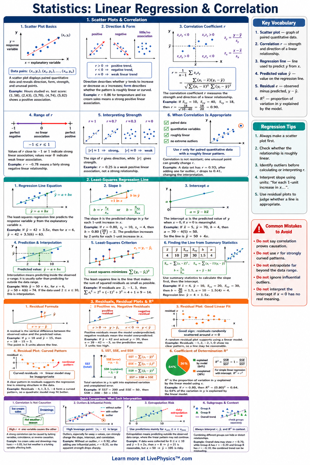
Linear regression and correlation describe relationships between two quantitative variables. This cheat sheet helps students read scatterplots, measure association, write prediction equations, and judge whether a model is reasonable. It is useful for homework, tests, labs, and data projects where students must connect calculations to real context. The main regression model is the least-squares line , where is the slope and is the intercept. Correlation measures the strength and direction of a linear relationship, while describes the proportion of variation explained by the model. Residuals, written , show prediction error and help check whether a linear model fits the data well.
Key Facts
- The least-squares regression line has the form , where is the predicted response, is the intercept, and is the slope.
- The slope of the regression line is , where is correlation and and are the sample standard deviations.
- The intercept is , so the regression line always passes through the point .
- The correlation coefficient is and satisfies .
- A residual is , and positive residuals mean the actual value is above the predicted value.
- The least-squares line minimizes the sum of squared residuals, written .
- The coefficient of determination is , which gives the proportion of variation in explained by the linear relationship with .
- Use a regression line for interpolation within the data range, but avoid extrapolation far outside the observed values.
Vocabulary
- Scatterplot
- A graph of paired quantitative data values used to show the form, direction, strength, and outliers in a relationship.
- Correlation coefficient
- The number that measures the direction and strength of a linear association between two quantitative variables.
- Least-squares regression line
- The line that minimizes the sum of squared residuals for a set of data.
- Residual
- A residual is the prediction error for one data point.
- Coefficient of determination
- The value is the proportion of variation in the response variable explained by the regression model.
- Extrapolation
- Extrapolation is using a regression model to predict values outside the range of the original data.
Common Mistakes to Avoid
- Using correlation to prove causation is wrong because a strong value of only shows linear association, not that one variable causes the other.
- Forgetting the context of the slope is wrong because means the predicted change in for each increase of unit in .
- Mixing up and is wrong because is an observed value, while is a predicted value from the regression line.
- Ignoring residual plots is wrong because a curved residual pattern suggests that a linear model may not be appropriate.
- Extrapolating far beyond the data is wrong because the linear pattern may not continue outside the observed range of values.
Practice Questions
- 1 A regression line is . What is the predicted value of when , and what does the slope mean in context?
- 2 For one data point, and . Find the residual and explain whether the prediction was too high or too low.
- 3 A data set has . Find and interpret what it says about the linear model.
- 4 A scatterplot shows a strong curved pattern, but the correlation is close to . Explain why a low correlation does not always mean there is no relationship.