SVD Image Compression Lab
The singular value decomposition writes any image as a sum of simple rank-1 layers, ordered from most important to least. Keep only the top few layers and you get a smaller image that still looks close to the original. Pick a sample image, slide the rank k, and watch the reconstruction, the compression ratio, and the singular value spectrum respond.
Guided ExperimentHow many singular values does a striped image need versus a noisy one?
You will compress the Stripes image and the Noise image with the same rank k. Predict which one reaches near-perfect reconstruction at a small k, and predict whether the noise image will ever look good at a rank that still saves storage.
Write your hypothesis in the Lab Report panel, then click Next.
Controls
Your image is downsampled to 48 × 48 grayscale in the browser and never uploaded to a server. Pick a sample above to switch back.
Original
48 × 48 pixelsRank-5 reconstruction
of 48 singular valuesThe reconstruction keeps only the largest k singular values and rebuilds the image from A_k = Σ sigma_i · u_i v_iᵀ. Raise k to recover more detail.
Singular value spectrum
Each bar is one singular value sigma_i, sorted largest to smallest. A fast drop toward zero means the image is close to low rank and compresses well. A long, slow tail means it needs many components.
Storage. The full image stores 2,304 numbers. Keeping the top 5 singular triplets stores only 485 numbers, which is k singular values plus k columns of U of length 48 plus k columns of V of length 48.
Eckart-Young theorem. Among all rank-5 matrices, this truncated SVD reconstruction is the best possible approximation of the original in both the Frobenius and spectral norms. No other rank-5 matrix can fit the image more closely, so the captured energy here is the most any rank-5 compression can achieve.
Data Table
(0 rows)| # | Sample | Rank k | Compression ratio | Energy % | Error % |
|---|
Reference Guide
The Singular Value Decomposition
Every matrix A can be factored as A = U Σ Vᵀ. Here U and V are orthogonal matrices whose columns are the left and right singular vectors, and Σ is diagonal holding the singular values sigma_1 ≥ sigma_2 ≥ ... ≥ 0.
- U. Left singular vectors, one column per component.
- Σ. The singular values, sorted from largest to smallest.
- V. Right singular vectors, one column per component.
Reading the factorization column by column turns the image into a weighted sum of outer products, A = Σ sigma_i · u_i v_iᵀ, each a single rank-1 layer.
Singular Values and the Spectrum
The singular values measure how much each layer contributes. The spectrum, a bar chart of sigma_i from largest to smallest, tells you at a glance how compressible the image is.
- Fast drop. The spectrum falls quickly toward zero, so the image is near low rank and compresses well.
- Long tail. The spectrum decays slowly, so many components are needed and compression is poor.
- Captured energy. The kept squared singular values over the total, a fraction from 0 to 1.
The Rank-k Approximation
Keeping only the first k layers gives the truncated SVD, A_k as the sum over the top k of sigma_i · u_i v_iᵀ. The Eckart-Young theorem says this is the best possible rank-k approximation of A in both the Frobenius and spectral norms.
- Storage. The full image needs m × n numbers, the rank-k version needs k × (m + n + 1).
- Compression ratio. The original count over the kept count, larger is more savings.
- Reconstruction error. The relative Frobenius norm of A minus A_k, the square root of one minus the captured energy.
Raising k recovers more detail at the cost of a smaller compression ratio. The best k balances quality against storage for the image at hand.
Where the SVD Is Used
The same truncation that compresses an image is one of the most widely used tools in applied mathematics and machine learning.
- Image compression. Keep the leading singular values to shrink an image with little visible loss.
- Principal component analysis. The SVD of centered data yields the principal directions.
- Latent semantic analysis. The truncated SVD of a term document matrix reveals hidden topics.
- Noise reduction. Dropping the small-sigma tail removes high-rank noise while keeping the signal.
In each case the leading singular directions hold the structure and the small ones hold the detail or noise that can be safely discarded.