Derivative & Integral Visualizer

Enter a function and see it alongside its derivative and integral. Drag a point along the curve to inspect the tangent line slope and the accumulated area. All computations run in your browser.

Quick answer

This visualizer plots a function with its derivative and antiderivative so students can connect tangent-line slope, rate of change, and accumulated signed area.

Study next

Enter a function

f(x) =

Presets

How to Read the Calculus Visualizer

Compare each curve at the same x-coordinate to connect function value, tangent slope, and accumulated signed change.

What the derivative means

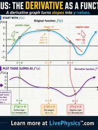
A derivative measures instantaneous rate of change. On the graph of a function, its value at a selected x-coordinate is the slope of the tangent line there. A positive derivative means the function is increasing locally, a negative derivative means it is decreasing, and a derivative of zero marks a horizontal tangent that may be a local maximum, a local minimum, or neither.

The derivative graph records those slopes as y-values. When the original curve becomes steeper upward, the derivative moves farther above zero; when the original curve falls more steeply, the derivative moves farther below zero. Units help preserve the meaning: if position is measured in meters and time in seconds, its derivative is measured in meters per second.

Derivative definition and notation

f'(x) = \lim_{h \to 0} \frac{f(x+h) - f(x)}{h}

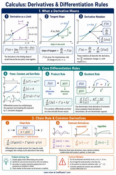
$f'(x)$ , $\frac{dy}{dx}$ , and $\frac{df}{dx}$ are common notations for the same derivative idea.

What the integral means

A definite integral measures accumulated signed change over an interval. Regions where the function is above the x-axis add to the accumulation, while regions below the axis subtract from it. This is why a definite integral is not always the same as total geometric area, which treats every region as positive.

An accumulation function starts at a chosen lower bound and gives the net integral up to each x-coordinate. Its graph rises where the original function is positive, falls where the original function is negative, and has a horizontal tangent where the original function is zero. The starting value depends on the chosen lower bound or constant, but the pattern of change depends on the original function.

Fundamental Theorem of Calculus

F(x) = \int_0^x f(t)\,dt

\frac{d}{dx}\int_0^x f(t)\,dt = f(x)

The theorem connects the two views: differentiating the accumulation function returns the original function. It also lets a definite integral be evaluated from any antiderivative by subtracting its values at the interval endpoints.

How to use the graph

Begin with a familiar function and predict the signs of its derivative before turning to the computed curve. Drag the inspection point slowly and compare the tangent line with the derivative value at the same x-coordinate. Then locate an interval where the original graph crosses the axis and watch how positive and negative contributions change the accumulated integral.

Use matching x-coordinates when comparing the three curves. Turning points on the original function should line up with zeros of the derivative, and local turning points on the accumulation curve should line up with zeros of the original function. Test a second function after you can explain those alignments in words rather than recognizing only the picture.

Differentiation rules used by the tool

Symbolic differentiation applies algebraic rules to produce an exact derivative formula. The visualizer combines these rules when the entered function contains products, quotients, or compositions.

Power rule

\frac{d}{dx} x^n = n x^{n-1}

Product rule

\frac{d}{dx}[f \cdot g] = f' \cdot g + f \cdot g'

Quotient rule

\frac{d}{dx}\left[\frac{f}{g}\right] = \frac{f' g - f g'}{g^2}

Chain rule

\frac{d}{dx} f(g(x)) = f'(g(x)) \cdot g'(x)

The integral curve is computed numerically, so it can approximate accumulation even when no elementary antiderivative exists. For example, $e^{-x^2}$ has no elementary closed-form antiderivative.

Common interpretation errors

Do not read the derivative's height as the original function's height. The derivative reports slope, so a function can sit high above the axis while having a derivative of zero. Likewise, a zero derivative is only a candidate for an extremum; a horizontal inflection point can have zero slope without changing from increasing to decreasing.

Do not assume an integral is negative whenever part of the curve lies below the axis. Compare the positive and negative signed contributions across the entire interval. Also distinguish an antiderivative from one definite accumulation function: antiderivatives differ by a constant, while fixing a lower bound chooses a particular starting value.

Finally, treat graphing and numerical output with appropriate precision. A narrow feature or discontinuity may be missed by a wide viewing window, and numerical integration is an approximation. Zoom, inspect nearby values, and verify domain restrictions before using the display as evidence for a conclusion.

Related Content

Sign in to save