Stock Market Statistics Lab
Investigate five years of daily price data across eight representative tickers. Compute log and simple returns, annualized volatility, Sharpe ratio, maximum drawdown, skewness, and excess kurtosis. Compare the empirical distribution of daily returns against a normal curve and inspect cross-asset correlation.
Guided Experiment Are Daily Returns Normal? Test for Fat Tails
If daily stock returns followed a normal distribution exactly, what fraction of days would you expect to see a move larger than 3 standard deviations? Compare your prediction against the actual count for a single ticker.
Write your hypothesis in the Lab Report panel, then click Next.
Controls
2 of 4 selected
Compare tickers on the same scale regardless of absolute price.
Price ChartNormalized = 100
Daily Returns Histogram (SPY)
Bars show observed daily-return density. Solid curve is the normal distribution with the same mean and standard deviation. Dashed red line marks the mean.
Stats by Ticker
| Ticker | Ann. Return | Ann. Vol | Sharpe | Max DD | Skew | Excess Kurt | N days |
|---|---|---|---|---|---|---|---|
| SPY | 31.65% | 22.87% | 1.209 | -43.86% | -0.952 | 5.402 | 1304 |
| QQQ | 21.69% | 34.86% | 0.507 | -71.78% | -0.807 | 4.342 | 1304 |
Annualized using 252 trading days. Sharpe uses the risk-free rate from the control panel. Excess kurtosis above 0 indicates fatter tails than a normal distribution.
Correlation Matrix (daily returns)
| SPY | QQQ | |
|---|---|---|
| SPY | 1.00 | 0.04 |
| QQQ | 0.04 | 1.00 |
Pearson correlation on daily returns over the intersection of dates. Green cells show positive correlation; red cells show negative correlation.
Data Table
(0 rows)| # | Ticker | Ann. Return (%) | Ann. Vol (%) | Sharpe | Max DD (%) | Skewness | Excess Kurt |
|---|
Reference Guide
Log Returns vs Simple Returns
Simple returns measure the percentage change in price across one period.
Log returns take the natural log of the price ratio. They are time-additive, which makes them more convenient for compounding analysis across many days.
For small daily changes the two are nearly identical, but log returns sum across days while simple returns do not.
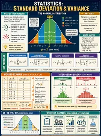
Annualized Volatility
Daily standard deviation of returns scaled to a one-year horizon. Assumes returns are independent across days (the random walk hypothesis).
252 is the typical number of trading days per year. Higher annualized volatility means larger expected daily swings.
Sharpe Ratio
Return per unit of risk. A higher Sharpe means more excess return for the same volatility.
Here R_f is the annualized risk-free rate (slider default 4%). The default rate is adjustable in the controls panel.
Maximum Drawdown
The largest peak-to-trough loss observed in the price series. A useful companion to volatility because it captures the worst experienced loss rather than just the dispersion.
Expressed as a negative fraction. For example, a drawdown of -33% means the price fell 33% from its prior high before recovering.
Skewness and Excess Kurtosis
Skewness measures asymmetry. A negative value means a longer left tail (large losses more likely than equally large gains).
Excess kurtosis measures tail heaviness relative to a normal distribution. A value above 0 means fat tails (extreme moves are more common than the normal model predicts).
For a perfectly normal distribution the excess kurtosis is 0. Daily stock returns typically show values between 3 and 15.
Random Walk Hypothesis
The random walk model treats each daily return as an independent draw from a normal distribution with constant mean and variance. Under this model future returns cannot be predicted from past returns.
The lab tests this model by comparing the empirical histogram to a fitted normal curve. Fat tails and skew indicate the model is incomplete.
About the Data
Daily closes covering 2020-01-02 through 2024-12-31 are synthesized in JavaScript using a seeded geometric Brownian motion. Regime parameters were tuned to match documented major moves (the 2020 COVID crash, the 2021 bull market, the 2022 bear market, the 2023 to 2024 rally, and the 2022 energy run-up).
For exact historical prices visit finance.yahoo.com or any data vendor. The synthetic dataset is suitable for educational analysis of return statistics, distribution shape, and correlation.