Watershed Explorer

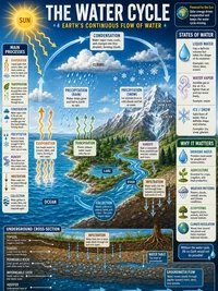
Explore the water cycle from precipitation to groundwater. Calculate water budgets using SCS curve numbers, visualize aquifer cross-sections with Darcy flow, model contaminant plume migration, and analyze well drawdown with the Theis equation.

Cross-Section View

Controls

Mode

Presets

Soil Type

Land Cover

Precipitation50 mm/day

Slope5 °

Results

P = I + R + ET

50.0 = 32.2 + 0.3 + 17.5 mm/day

Infiltration

32.2 mm/day

64%

Runoff

0.3 mm/day

Evapotranspiration

17.5 mm/day

35%

SCS Curve Number

Water Budget Components

Reference Guide

Darcy's Law

Darcy's Law describes the flow of fluid through a porous medium. The specific discharge (Darcy velocity) is proportional to the hydraulic gradient.

v = -K \frac{dh}{dl}

Where $K$ is hydraulic conductivity (m/day), and $dh/dl$ is the hydraulic gradient. The actual pore velocity is $v_s = v/n$ where $n$ is porosity.

Water Budget

The water budget partitions precipitation into infiltration, surface runoff, and evapotranspiration.

P = I + R + ET

Runoff is estimated using the SCS Curve Number method, where $S = \frac{25400}{CN} - 254$ is the maximum soil retention and $Q = \frac{(P - 0.2S)^2}{P + 0.8S}$ for $P > 0.2S$ .

Theis Equation

The Theis equation gives the drawdown at distance r from a pumping well in a confined aquifer.

s = \frac{Q}{4\pi T} W(u), \quad u = \frac{r^2 S}{4Tt}

For small $u$ (large time or small distance), the Cooper-Jacob approximation gives $W(u) \approx -0.5772 - \ln(u)$ .

Contaminant Dispersion

A contaminant plume spreads by advection (bulk flow) and dispersion (mixing). The 2D Gaussian solution describes concentration in space and time.

C(x,y,t) = \frac{C_0}{4\pi t \sqrt{D_L D_T}}\, e^{-\frac{(x-vt)^2}{4D_Lt} - \frac{y^2}{4D_Tt}}

The dispersion coefficients are $D_L = \alpha_L v$ (longitudinal) and $D_T \approx 0.1 D_L$ (transverse), where $\alpha_L$ is dispersivity.