Click image to open full size
Residuals & Residual Plots Cheat Sheet
A printable reference covering residuals, predicted values, residual plots, least-squares regression, and pattern interpretation for grades 10-12.
Related Tools
Related Labs
Related Worksheets
Related Infographics
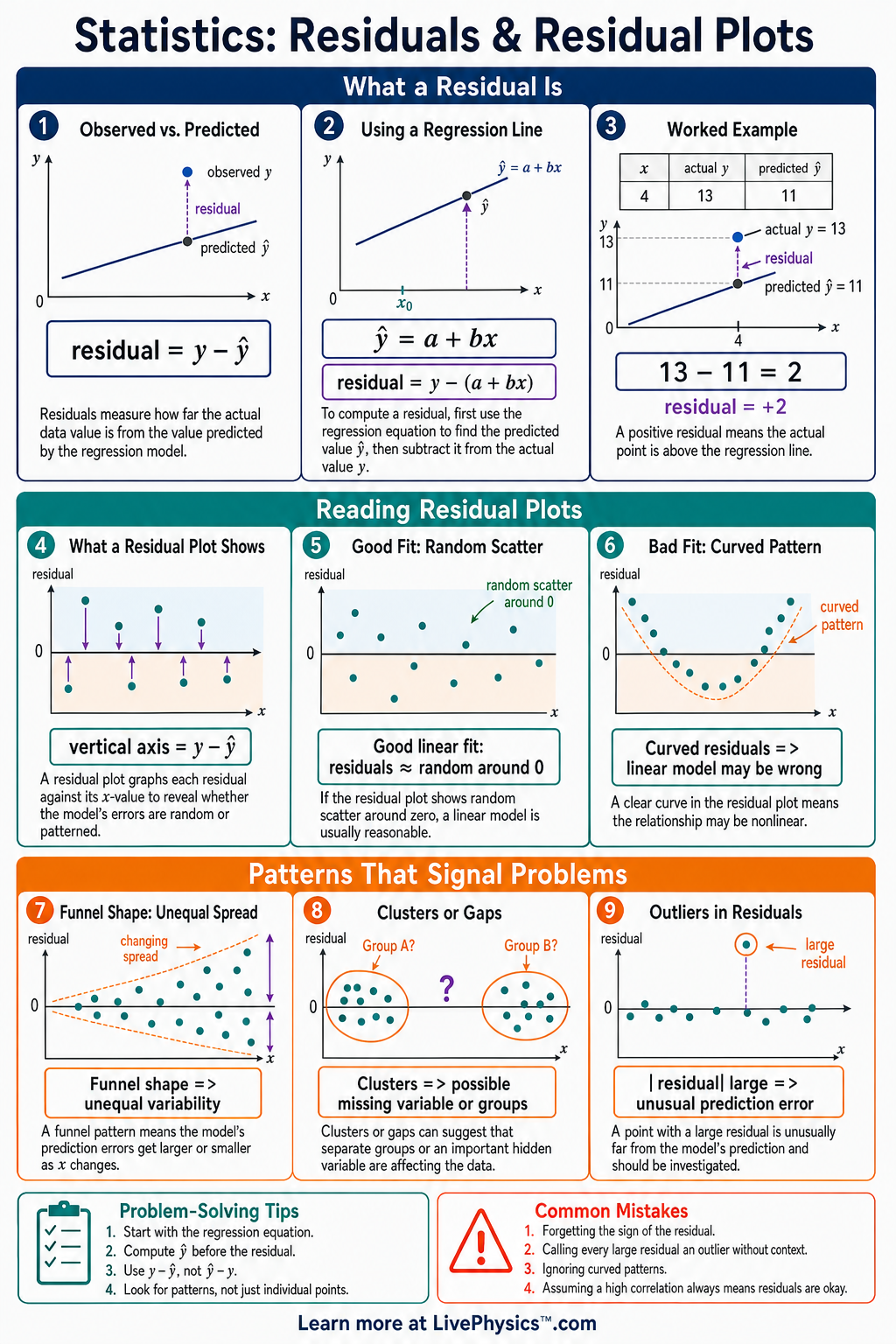
Residuals measure how far each observed data value is from the value predicted by a regression model. This cheat sheet helps students calculate residuals, build residual plots, and decide whether a linear model is reasonable. Residual plots are important because they reveal patterns that a scatterplot or correlation value may hide. Students use them to check model fit, spot outliers, and compare predictions to real data. The main formula is , where is the residual, is the observed value, and is the predicted value. A residual plot places the explanatory variable on the horizontal axis and the residuals on the vertical axis. A good linear model usually has residuals randomly scattered around . Curved patterns, changing spread, or extreme points suggest the model may not be appropriate.
Key Facts
- A residual is calculated using , where is the observed value and is the predicted value.
- A positive residual means the observed value is above the regression line because .
- A negative residual means the observed value is below the regression line because .
- For a least-squares regression line, the residuals always have a sum of , up to rounding error.
- A residual plot graphs each point as , using the original explanatory variable and the residual .
- A residual plot with random scatter around supports using a linear model.
- A curved pattern in a residual plot suggests that a nonlinear model may fit the data better than a line.
- A fan-shaped residual plot shows nonconstant spread, meaning prediction errors change size as changes.
Vocabulary
- Residual
- A residual is the difference between an observed response value and the value predicted by a model, calculated as .
- Predicted Value
- A predicted value, written , is the response value estimated by a regression equation for a given .
- Residual Plot
- A residual plot is a graph of residuals against the explanatory variable, usually shown as points .
- Least-Squares Regression Line
- A least-squares regression line is the line that minimizes the sum of squared residuals, .
- Outlier
- An outlier is a data point with an unusually large residual or an unusual position compared with the rest of the data.
- Nonlinear Pattern
- A nonlinear pattern occurs when residuals show a curve or systematic shape instead of random scatter around .
Common Mistakes to Avoid
- Reversing the residual formula is wrong because gives the opposite sign; use .
- Thinking a high correlation always means a good linear model is wrong because a residual plot can reveal curvature or changing spread.
- Ignoring the sign of a residual is wrong because positive residuals mean the point is above the line and negative residuals mean it is below the line.
- Using instead of on the vertical axis of a residual plot is wrong because the plot must show prediction errors, not original response values.
- Calling any large residual an error in the data is wrong because an outlier may be real and should be investigated before being removed.
Practice Questions
- 1 A regression model predicts for a data point with observed value . Find the residual .
- 2 For the regression equation , find the residual when and the observed value is .
- 3 A point has residual and predicted value . Find the observed value .
- 4 A residual plot shows a clear U-shaped pattern around . Explain what this suggests about using a linear model for the data.