Weather and Pressure Visualizer

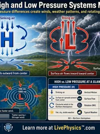
Atmospheric pressure is the weight of the air column above a given point. It is measured in hectopascals (hPa), where standard sea-level pressure is 1013.25 hPa.

A High pressure system (anticyclone) has denser, descending air and fair weather. A Low pressure system (cyclone or depression) has rising air, clouds, and precipitation.

The pressure difference between systems drives wind. Air flows from high to low pressure, but the Coriolis effect and friction deflect it, producing circular wind patterns.

High in the atmosphere, friction is negligible. Wind reaches geostrophic balance when the pressure gradient force exactly balances the Coriolis force.

Here f is the Coriolis parameter, rho is air density (1.225 kg/m³), and dP/dx and dP/dy are the east-west and north-south pressure gradients. Geostrophic wind flows parallel to isobars, not across them.

Earth's rotation deflects moving air to the right in the Northern Hemisphere and to the left in the Southern Hemisphere. This is the Coriolis effect.

Omega = 7.292 x 10^-5 rad/s is Earth's rotation rate and phi is latitude. At the equator f = 0 (no deflection), and the effect strengthens toward the poles.

Result: Lows rotate counterclockwise in NH (cyclonic), clockwise in SH. Highs rotate clockwise in NH (anticyclonic), counterclockwise in SH.

Jet streams are fast, narrow air currents in the upper troposphere (around 10-12 km altitude) flowing west to east at 50-300 km/h. They form at the boundary between cold polar air and warm tropical air.

There are two main jet streams in each hemisphere:

• Polar jet stream (60 degrees latitude) - strongest in winter
• Subtropical jet stream (30 degrees latitude) - more consistent year-round

Jet streams are not straight - they meander in Rossby waves. Where the jet dips south (trough) brings cold air; where it bulges north (ridge) brings warm air.

Meteorologists analyze surface pressure maps to predict weather. Key rules of thumb:

• Tightly packed isobars indicate strong winds
• Falling barometric pressure signals approaching storms
• Rising pressure signals clearing skies
• Lows bring clouds and rain as air rises and cools
• Highs bring clear, dry weather as air descends and warms

Modern numerical weather prediction solves the Navier-Stokes equations over a global grid. The primitive equations form the core, including geostrophic balance, hydrostatic approximation, and thermodynamic energy equations.

The map starts with three default systems: an Atlantic High, the Iceland Low, and a Pacific High. These approximate typical Northern Hemisphere winter patterns.

• Click any pressure center to select it and see its stats
• Use Add H or Add L, then click the map to place new systems
• Click Remove to delete the selected system
• Toggle Wind to show or hide animated geostrophic wind particles
• Toggle Jet Stream to show the simplified jet stream overlay
• Use Share to copy a link with your current configuration

Wind particles follow real geostrophic wind calculations, responding to pressure gradients and the Coriolis parameter at each latitude.