Food Web Investigation Guide
Use the model to make a prediction, change one condition, and explain the resulting energy-transfer pattern with evidence.
Trophic levels and the 10% rule
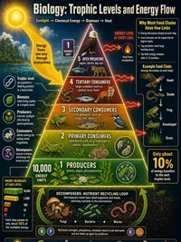
A trophic level describes an organism's feeding position, not simply its size. Producers capture energy and form the base, primary consumers eat producers, secondary consumers eat primary consumers, and tertiary consumers feed higher in the web. Omnivores may connect more than one level because their position changes with what they eat.
The 10% rule is a useful estimate: roughly one tenth of the energy stored as biomass at one level becomes biomass available to the next. The rest supports respiration, movement, maintenance, and other life processes or leaves as waste and heat. Transfer efficiency varies among organisms and ecosystems, so treat 10% as a model to test rather than an exact law.
Energy transfer model
Here, ε is the transfer efficiency. A consumer's energy budget can also be written as input energy divided among respiration, growth, and waste.
Only growth, the new biomass represented by G, can become food energy for the next trophic level.
How to run the investigation
- Choose an ecosystem, keep every species active, and run the model with the default producer energy. Use the automatically recorded energy values as the baseline trial. Copy the baseline table as CSV or use Export CSV before resetting; Reset clears the in-tool table rows.
- Reset, then remove a consumer or predator species while keeping producer energy fixed. Predict which energy connection disappears first and how energy reaching higher trophic levels may change. Run for the same duration, then copy or export the treatment rows before the next reset.
- For a separate bottom-up experiment, reset again and use the producer-energy control to change the energy entering the web. Keep all species active so this trial tests one control variable. Copy or export its completed table before any later reset.
- Compare the saved or exported rows at equivalent time steps. Use the in-tool energy visualization to explain differences during each run, and repeat a setup before testing another removal or energy level.
Real-ecosystem context, trophic cascades and stability
In real ecosystems, a trophic cascade begins when a change in one population affects organisms at other feeding levels. Losing a top predator can release prey from control, and the additional feeding by that prey can affect organisms lower in the web. Bottom-up cascades can begin when the energy entering through producers changes and less food energy reaches consumers.
This lab represents food-web connections and energy transfer after a consumer or predator is removed, but it does not simulate population sizes or prey release. Use the cascade concept as real-ecosystem context for the energy investigation, not as a population result produced by the model. Food webs may resist disturbance when consumers have alternate energy pathways, while the loss of a highly connected or keystone species can have a larger real-world effect.
Reading results and making a safe conclusion
Compare saved or exported rows at equivalent time steps from the baseline and treatment trials. During each run, use the energy visualization to trace active links, check the energy at each trophic level, and preserve the data table's recorded time steps before resetting. A consistent difference in several matching records is stronger evidence than one temporary rise or fall.
For a removal trial, trace which energy links disappear and which higher levels receive less energy. For a producer-energy trial, look for the change to begin at the producer level and continue upward through consumers. Repeat the same setup before deciding that the pattern is stable.
Interpret the output as evidence from a simplified energy model, not as a guaranteed forecast for an ecosystem. Real populations are also shaped by weather, disease, migration, habitat quality, reproduction, competition, and time delays that this lab does not calculate. A safe conclusion names the ecosystem, control setting, changed variable, recorded energy evidence, and limits of the model.