Radiative Balance & Greenhouse Explorer

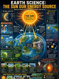
The Sun delivers about 1361 W/m² at Earth's distance. Averaged over Earth's spherical surface, the incoming solar flux is S/4 = 340 W/m².

About 30% is reflected back to space (albedo = 0.30), so Earth absorbs roughly 238 W/m². At equilibrium, the planet must radiate the same amount back to space.

The difference between surface emission (~390 W/m²) and top-of-atmosphere emission (~238 W/m²) is the greenhouse effect, which traps about 152 W/m² of infrared radiation.

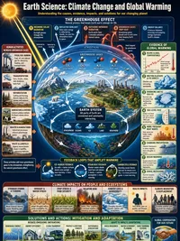
Without greenhouse gases, Earth's surface would be about 255 K (−18°C). The actual average is about 288 K (15°C), a 33°C warming caused by CO₂, H₂O, CH₄, N₂O, and other gases that absorb and re-emit infrared radiation.

Here $\sigma = 5.67 \times 10^{-8}$ W m⁻² K⁻⁴ is the Stefan-Boltzmann constant and $\varepsilon$ is the effective emissivity. Lower emissivity means the atmosphere traps more outgoing radiation, raising the equilibrium temperature.

Radiative forcing measures how much a change in atmospheric composition shifts the energy balance. The IPCC simplified formula for CO₂ is

Doubling CO₂ from 280 to 560 ppm gives $\Delta F \approx 3.7$ W/m², which translates to roughly 3°C of warming using a climate sensitivity of $\lambda \approx 0.8$ °C per W/m².

Methane and N₂O follow square-root relationships, reflecting the saturation of their absorption bands at higher concentrations.

The equilibrium climate sensitivity (ECS) describes how much warming results from doubled CO₂ after all feedbacks reach equilibrium. Current estimates range from 2.5°C to 4.0°C.

Key feedback loops amplify the initial warming. Water vapor feedback roughly doubles the response because warmer air holds more water vapor, itself a potent greenhouse gas. Ice-albedo feedback reduces reflectivity as ice melts, absorbing more solar energy. Together, these positive feedbacks amplify the bare forcing response by about a factor of 2 to 3.